4 Working With Data

You can download the demo data files fro various types from the link below:-

4.1 Importing Data into R

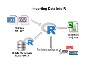
4.1.1 Import flat files (`.csv`, `.txt` )

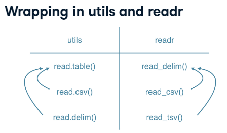
read.table() is the main function
read.csv() wrapper for CSV
read.delim() wrapper for tab-delimited files

# install th read r package
install.packages(readr)
# load the read r package
library(readr)
# read csv file using read.table()
df1 <- read_csv("data/demo csv data.csv", show_col_types = FALSE)
# read txt file that doesnot headers
df2 <- read_delim("data/demo data text.txt")
# Or use
df3 <- read_tsv("data/demo data text.txt")

4.1.2 Import Excel data file

# install package
install.packages("readxl")
# load package
library(readxl)
# by default, it loads the first sheet
excel_data <- read_excel("data/demo excel data.xlsx")
# if the excell workbook has many sheets and you want to
# load a specific one, e,g, sheet two
excel_data <- read_excel("data/demo excel data.xlsx", sheet = 2)

4.1.3 Import STATA data file

install.packages("readstata13")
library(readstata13)
stata_data <- read.dta13("data/demo stata data.dta", generate.factors = TRUE)

4.1.4 Importing R data file

load("data/demo R data.rda")

4.1.5 Importing Web data file

Data on the web comes in several modes, for example:

files that you can download
APIs
content such as HTML tables
custom data browsers
and more.

However, for this section, let us keep it basic, If interested is the other option, contact the author for some materials OR code that might not be in this book.

4.1.6 Inbuilt Datasets

To see the list of pre-loaded datasets, type the function data()

# Loading
data(mtcars)
# learn more about the data
`?`(mtcars)
# OR
help(mtcars)

In case you want to get a list of datasets in a specific R package using data()

# list available datasets in ggplot2 package
data(package = "ggplot2")

4.1.7 Other file formats

File Type	File extension	function	package
Database file type	.dbf	read.dbf()	foreign
SPSS data file	.sav	read_spss()	haven
SQL Database		dbConnect() dbGetQuery()	DBI, RMySQL, RPostgreSQL, ROracle depending on the specific database
SAS data file	.xport	read_sas()	haven
Matlab file		readMat()	R.matlap

4.2 Explore the dataset

In R,There are various functions to explore a data frame. These functions can help you get a better understanding of the structure and contents of your data frame.

Here are some common functions.

head() - shows the first few rows of the data frame

tail() - shows the last few rows of the data frame

str() - displays the structure of the data frame

summary() - provides summary statistics for each variable in the data frame

nrow() - returns the number of rows in the data frame

ncol() - returns the number of columns in the data frame

colnames() - returns the names of the columns in the data frame

row.names() - returns the names of the rows in the data frame

unique() - returns unique values in a column of the data frame
view() - shows the dataset in spreadsheet form
dim() - returns the dimensions of the data frame as a vector of two integers, the number of rows and the number of columns
is.na() - returns a logical vector indicating whether each value in the data frame is missing or not

For a better visual display of the results, additional packages can be used such as skimr, gtsummary, kable, as it will be in the preceding sections of this guide, however, below is a sneak peak of the basic ones.

install.packages("skimr")
library(skimr)
# get the summary of all the variable, alternative to
# ---str()---
skim(iris)

4.3 Pull basic statistics from your data

4.3.1 For continuous variables:

mean() - calculates the mean of a numeric vector

mean(numeric_vector)

median() - calculates the median of a numeric vector

median(numeric_vector)

sd() - calculates the standard deviation of a numeric vector

sd(numeric_vector)

var() - calculates the variance of a numeric vector

min() - returns the minimum value of a numeric vector

max() - returns the maximum value of a numeric vector

range() - returns the range of a numeric vector as a vector of length 2 containing the minimum and maximum values

quantile() - calculates the quantiles of a numeric vector

summary() - provides summary statistics for a numeric vector, including the minimum, 1st quartile, median, mean, 3rd quartile, and maximum
Simple plots using the base package

# Histogram:
hist(data$variable_name)
# Boxplot:
boxplot(data$variable_name)
# Density Plot:
plot(density(data$variable_name))
# Scatterplot:
plot(data$variable_name1, data$variable_name2)

For categorical/character variables:

table() - creates a contingency table of the frequencies of the levels of a categorical variable

prop.table() - converts a contingency table of frequencies to a contingency table of proportions

summary() - provides a summary of a factor variable, including the number of levels and the frequency of the most common level.
Simple plot using the base package

# Bar Plot:
barplot(table(data$variable_name))
# Pie Chart:
pie(table(data$variable_name))
# Stacked Bar Plot:
barplot(table(data$variable_name, data$grouping_variable), col = c("red",
    "blue"))

4.4 Exporting Data from R

save(data_object, file = "my_data.rda")  # exporting R data object
write.csv(data_object, file = "my_data.csv")  # exporting csv data file
write.table(data_object, file = "my_data.txt")  # exporting text data file
writexl::write_xlsx(data_object, file = "my_data.rda")  # exporting excel data file
jsonlite::write_json(data_object, file = "my_data.json")  # exporting java script data file
xml2::write_xml(data_object, file = "my_data.xml")  # exporting to xml file
haven::write_sas(data_object, file = "my_data.xport")  # exporting SAS data file
haven::write_dta(data_object, file = "my_data.dta")  # exporting STATA data file
haven::write_sav(data_object, file = "my_data.sav")  # exporting SPSS data file

You can download the demo data files fro various types from the link below:-

CLICK here to open the datasets folder

4.5 Tasks

4.5.1 Exercise 1

Import a CSV file named “sales_data.csv” into RStudio.

NOTE: You can download the sales data to your computer from; Click here Download the Sales Data
Export the data in the “sales_data” object as a CSV file named “sales_data_export.csv”.
Using the “summary” function, extract basic statistics (mean, median, minimum, maximum) for the “sales_data” object.
Load a new data file named “customer_data.xlsx” into RStudio.
Explore the data by using the “head” and “tail” functions to view the first and last few rows of the data.
Use the “str” function to display the structure of the “customer_data” object.
Pull basic statistics (mean, median, minimum, maximum) for the “customer_data” object using the “summary” function.
Export the data in the “customer_data” object as a CSV file named “customer_data_export.csv”.

4.5.2 Exercise 2

Import the inbuilt data of iris into RStudio.

Using the “plot” function, create a scatter plot of the “Sepal.Length” and “Sepal.Width” columns in the “iris” object.
Using the “boxplot” function, create a box plot of the “Petal.Length” column in the “iris” object, grouped by the “Species” column.
Using the “hist” function, create a histogram of the “Petal.Width” column in the “iris” object, grouped by the “Species” column.
Using the “plot” function, create a line plot of the “Sepal.Length” column in the “iris” object, grouped by the “Species” column.

3 Operators & Data Objects

5 Data Wrangling