9 Reproducible Results (Markdown, Quarto & Notebooks)
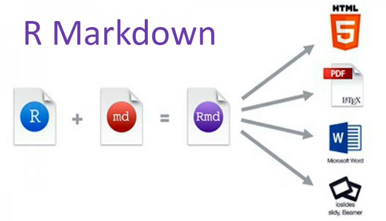
Welcome to this chapter on reproducible results in R! In this chapter, we will explore the different tools and techniques that you can use to ensure that your data analysis workflows are not only accurate but also reproducible. We’ll be covering Markdown, Quarto, and Notebooks , so you can get a comprehensive understanding of each one.

Although we will cover all three tools - R Markdown, R Notebooks, and Quarto - we will put a particular emphasis on R Markdown. This is because R Markdown is one of the most widely used for creating reproducible documents and presentations in R.
Most Importantly! Knowing how to use R Markdown can be a great foundation for learning and using R Notebooks and Quarto. This is because R Markdown is often considered the simplest and most user-friendly of the three tools, making it an excellent starting point for those new to reproducible data analysis. Once you have a solid understanding of R Markdown, you’ll likely find it easier to pick up the more advanced features of R Notebooks and Quarto. Plus, since R Markdown documents can easily be converted to R Notebooks or Quarto files, having a strong understanding of R Markdown can make it easier to transition to the other tools. So, even if you ultimately decide to use a different tool for your particular use case, learning R Markdown is definitely a great starting point.
9.1 Why Reproducibility
Before we dive into the specifics, let’s take a step back and ask why reproducibility is so important in the first place. In today’s data-driven world, many important decisions are made based on data analyses. But how can we be sure that these analyses are accurate and reliable? One way to increase confidence in our results is to make sure that our analyses are reproducible. This means that anyone can take our code and data, run it themselves, and get the same results that we did. Not only does this increase confidence in our results, but it also makes it easier to share our work with others and build on it collaboratively.
So, let’s start by exploring R Markdown, one of the most popular tools for creating reproducible documents and presentations in R. With R Markdown, you can combine code, text, and figures in a single document, making it easy to create a narrative around your analysis. We’ll show you how to create simple documents, as well as more complex reports with multiple outputs.
Next up, we’ll dive into R Notebooks, another powerful tool for creating reproducible analyses. With R Notebooks, you can create interactive documents that allow readers to explore your data and code in real-time.
Finally, we’ll introduce you to Quarto, a newer tool for creating reproducible reports and documents. Quarto builds on the strengths of both R Markdown and Notebooks, allowing you to create complex, interactive reports with a variety of outputs.
Throughout the chapter, we’ll provide examples and best practices for using each tool, as well as tips and tricks for making your analyses more reproducible. By the end of this chapter, you’ll have a solid understanding of the different tools available for creating reproducible results in R, and be able to choose the best tool for your specific needs.
So let’s get started and dive into the world of reproducible data analysis in R!
9.2  The Visual Editor
If you’re not comfortable with writing Markdown or LaTeX code, don’t worry - there is a visual editor available for R Markdown, Quarto, and R Notebooks. This editor provide a point-and-click interface that makes it easier to create and edit your documents. Isn’t that nice ?!…

Starting with R Studio 1.4 (i.e. release of January 2021 and later ), the IDE includes a visual markdown editor that works on any markdown-based document, such as .md or .Rmd or .Qmd files.
Highlights of visual mode include:
Visual editing for all of Pandoc markdown, including tables, divs/spans, definition lists, attributes, etc.
Extensive support for citations, including integration with Zotero and the ability to insert citations from DOIs or searches of PubMed, Crossref, and DataCite.
Scientific and technical writing features, including cross-references, footnotes, equations, code execution, and embedded LaTeX.
Writing productivity features, including real time spell-checking and outline navigation.
Tight integration with source editing (editing location and undo/redo state are preserved when switching between modes).
Rich keyboard support. In addition to traditional shortcuts, you can use markdown expressions (e.g.
##,**bold**, etc.) for formatting. If you don’t remember all of the keyboard shortcuts, you can also use the catch-all⌃ /shortcut to insert anything.
Let me walk you through several features of visual editing mode.
- To switch into the visual mode for a markdown document:
In
RStudio v2022.02, click the “Visual” button located on the left side of the editor toolbar.In earlier versions, click the compass icon located on the right side of the editor toolbar.
Alternatively, use the Ctrl + Shift + F4 keyboard shortcut.
- You can customize various editor settings. Go to
Tools->Global Options->R Markdown->Visualto choose your options, such as:
Whether your new documents use the visual markdown editor by default.
Whether the document outline shows by default.
How to wrap text in the document.
<img src="images/visual_editor_tools.png" width="90%" style="display: block; margin: auto;" />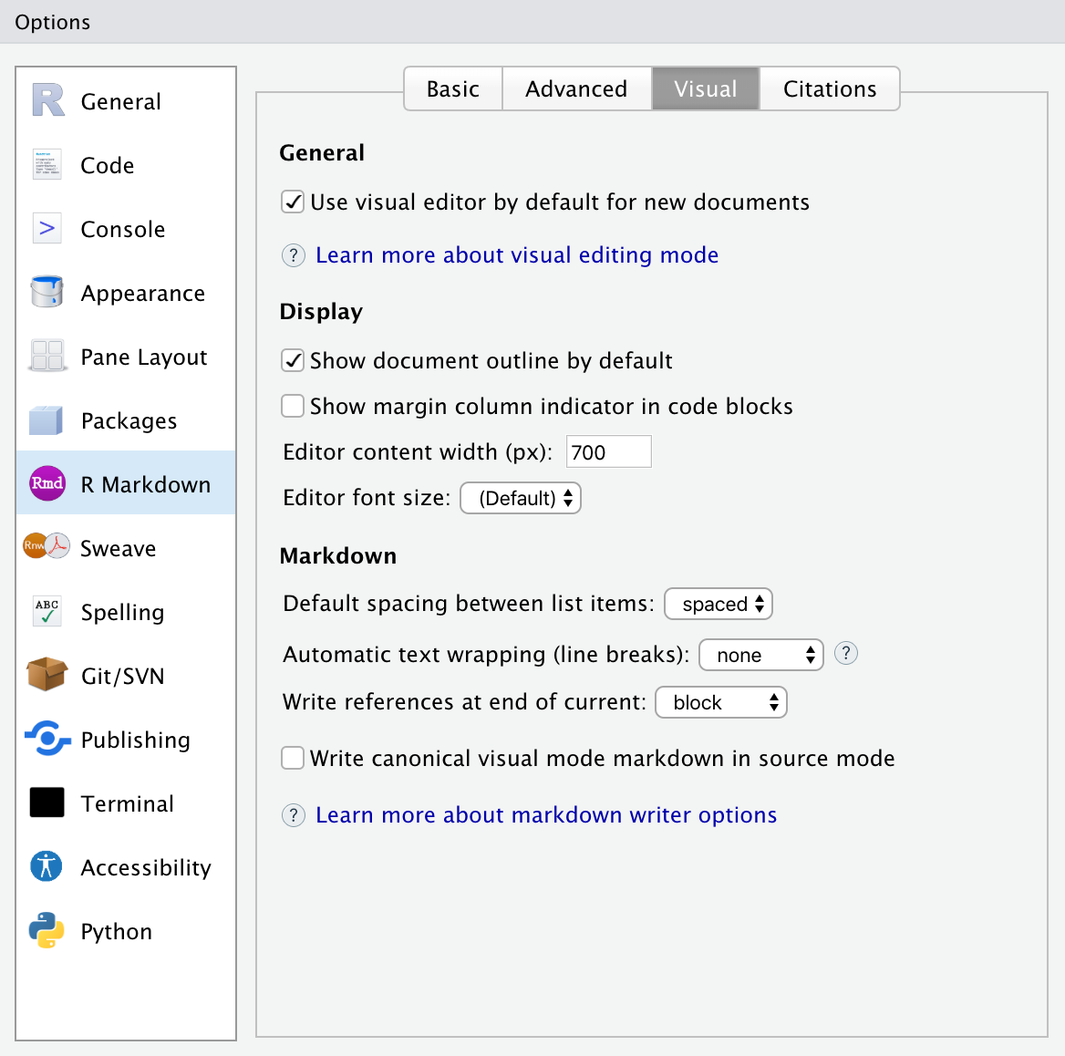
To explore more about the Visual Editor, CLICK HERE
9.3 R Markdown
Welcome to the exciting world of reproducible data analysis using R markdown! In this section, we’ll explore the powerful tool of R Markdown and how it can help you create top-notch, reproducible reports to facilitate open science.
9.3.1 What is R markdown?
R Markdown is a versatile tool that allows you to seamlessly combine code, text, graphics, and tables into a single document. Not only does this make your workflow more streamlined, but it also ensures that your analysis can be easily reproduced by others. So what are you waiting for? Let’s dive in and discover the exciting possibilities of R Markdown!
R markdown is a simple and easy to use plain text language used to combine your R code, results from your data analysis (including plots and tables) and written commentary into a single nicely formatted and reproducible document (like a report, publication, thesis chapter or a web page like this one).
In technical terms, R Markdown is a type of markup language, which is essentially a way to create a plain text file that can include formatted text, images, headers, and links to other documents. Markdown is the underlying language that R Markdown is based on, and it’s widely used for creating easily readable documents on the web. You’ve likely encountered another markup language, HTML, without even realizing it, as it’s the backbone of most web content today.
But fear not, learning R Markdown is a breeze, and it’s far simpler than HTML. Plus, when used with RStudio, it seamlessly integrates into your workflow, allowing you to create content that’s loaded with features and visually appealing. So why not take advantage of this powerful tool? Don’t worry about the details just yet.
At this point, it’s likely that you’re already using R to delve into and scrutinize your intriguing data. This means that you’re already on the path towards making your analysis more transparent, reproducible, and easily shared with others.
If i guess right, you might be currently doing this (below)?
You importing data from your preferred source into RStudio, write R code to explore and analyze the data, and then manually combining plots, analysis output tables, and written prose into a single MS Word document, for your report.

 While this approach isn’t necessarily wrong, it has its limitations……..
Firstly, it’s not very reproducible. By separating your R code from the final document, you’re creating multiple opportunities for undocumented decisions to be made, such as which plots to use or which analyses to include/exclude.
Secondly, it’s inefficient. If you need to make changes later on (such as creating a new plot or updating your analysis), you’ll have to create or modify multiple documents, increasing the chances of mistakes creeping into your workflow.
Thirdly, it’s challenging to maintain. If your analysis changes, you’ll need to update multiple files and documents.
Lastly, it can be difficult to decide what to share with others. Should you share all of your code (including data exploration and model validation), or just the code specific to your final document? Many researchers maintain two R scripts, one for analysis and one for sharing with their final report. However, this practice is time-consuming and confusing, and should be avoided.
To address these limitations, we’ll explore a more efficient and reproducible workflow using R Markdown, R Notebooks, and Quarto in the following chapters of this book. With these tools, you can seamlessly combine your R code, written prose, plots, and analysis output in a single document that’s easy to share and maintain, making your research more robust and efficient.
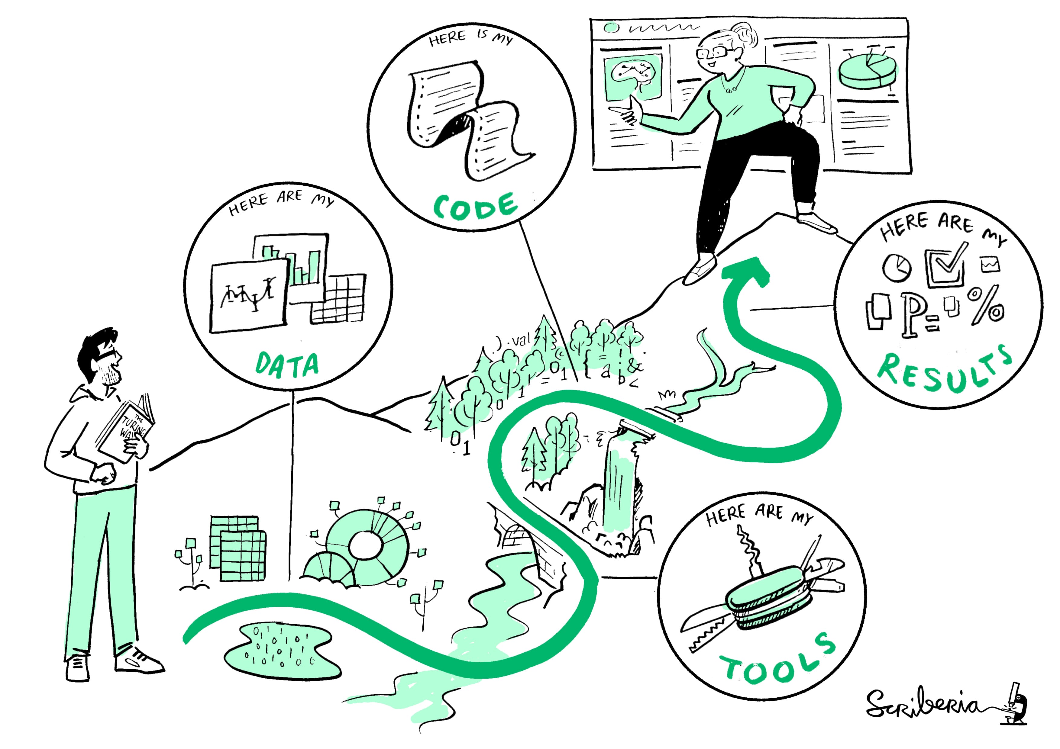
Your data is imported into RStudio (or R) as before but this time all of the R code you used to analyse your data, produce your plots and your written text (Introduction, Materials and Methods, Discussion etc) is contained within a single R markdown document which is then used (along with your data) to automatically create your final document. This is exactly what R markdown allows you to do.
R Markdown is a powerful tool that offers many advantages to data analysts and researchers.
One of the primary benefits of using R Markdown is that it explicitly links your data with your R code and output, creating a fully reproducible workflow. This means that all of the R code used to explore, summarize, and analyze your data can be included in a single, easy-to-read document.
Another advantage of R Markdown is its versatility. With just a single R markdown document, you can create a wide variety of output formats, including PDFs, HTML web pages, and Microsoft Word documents, among many others. This makes collaboration and communication with others a breeze.
R Markdown also enhances the transparency of your research. By including your data and R markdown file with your publication or thesis chapter as supplementary material or hosting it on a GitHub repository, you can provide others with a clear and complete picture of your research process.
Finally, R Markdown can significantly increase the efficiency of your workflow. If you need to modify or extend your current analysis, you can simply update your R markdown document, and these changes will automatically be included in your final document. This not only saves time but also ensures that your analyses are always up-to-date and accurate.
9.3.2 Get started with R markdown
To use R markdown you will first need to install the rmarkdown package and any package dependencies. If you would like to create pdf documents (or MS Word documents) from your R markdown file you will also need to install a version of LaTeX on your computer. If you’ve not installed LaTeX before, we recommend that you install TinyTeX Again.
9.3.3 Create an R markdown document
Right, time to create your first R markdown document. Within RStudio, click on the menu File -> New File -> R Markdown.... In the pop up window, give the document a ‘Title’ and enter the ‘Author’ information (your name) and select HTML as the default output. We can change all of this later so don’t worry about it for the moment.
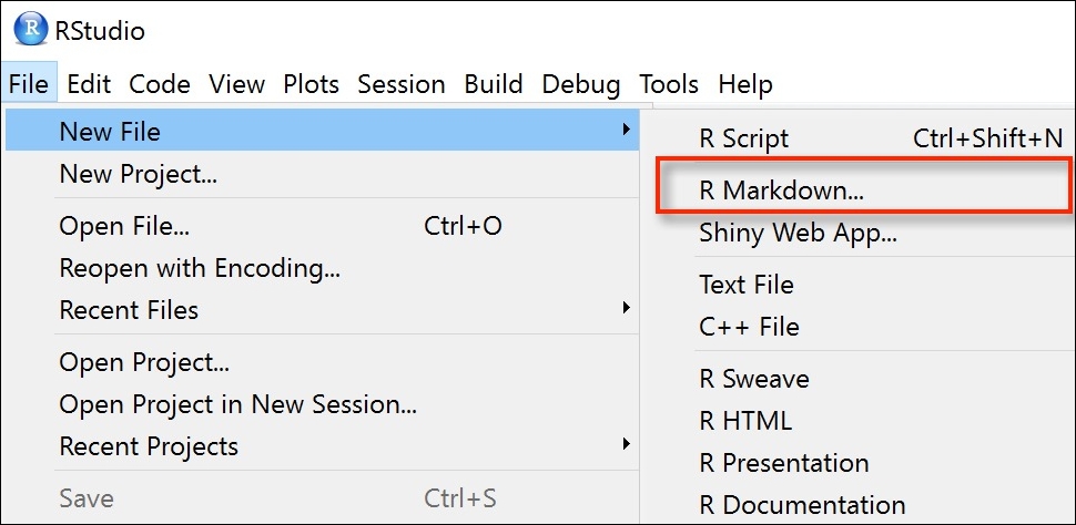
As you begin creating a new R Markdown document, you may notice that it comes with some pre-existing code examples. Typically, you would remove all of this code except for the important information at the top, which is known as the YAML header (we’ll delve more into that shortly), and start adding your own code.
For now, though, let’s use this document as a practice exercise for converting R Markdown to both HTML and PDF formats. By doing so, we can ensure that everything is functioning as it should be before diving into more advanced coding techniques.
After you’ve finished creating your R Markdown document, it’s important to save it in a location that’s easy to find. You can easily save your document by clicking on “File” in the RStudio menu and selecting “Save” (or by using the keyboard shortcut “Ctrl + S" on Windows or”Cmd + S” on a Mac). Don’t forget to give your file an appropriate name. Keep in mind that your new R Markdown file will have a .Rmd file extension.
To transform your .Rmd file into a polished HTML document, simply click on the drop down next to the “Knit” icon at the top of your source window. From there, select “Knit to HTML” to create a formatted, HTML version of your document. Notice that there is a new R Markdown tab in your console window which provides you with information on the rendering process and will also display any errors if something goes wrong.
If everything went smoothly a new HTML file will have been created and saved in the same directory as your .Rmd file (ours will be called file_name.html). To view this document simply double click on the file to open in a browser (like Chrome or edge) to display the rendered content. RStudio will also display a preview of the rendered file in a new window for you to check out (your window might look slightly different if you’re using a Windows computer).

Great, you’ve just rendered your first R markdown document. If you want to knit your .Rmd file to a pdf document then all you need to do is choose knit to PDF instead of knit to HTML when you click on the knit icon. This will create a file called file_name.pdf which you can double click to open. Give it a go!
9.3.4 The R markdown anatomy
Great, now that you can easily convert your R markdown file into both HTML and PDF formats in RStudio, let’s delve deeper into the key components that make up a typical R markdown document. Typically, an R markdown document comprises of three main elements:
YAML header,
Formatted text, and
one or more code chunks.
By mastering these components, you’ll be able to create powerful and effective data analyses that are both informative and visually appealing.
9.3.4.1 YAML header
YAML stands for “YAML Ain’t Markup Language”, and it’s a human-readable data serialization language.
The YAML header is an optional component that appears at the top of an R Markdown document and is enclosed by three hyphens (
---) on a line of its own before and after.The YAML header contains metadata and options for the entire document, such as the title, author, date, output format, and more.
A minimal YAML header is automatically generated by RStudio when you create a new R Markdown document, but you can modify it to suit your needs.
The most commonly used YAML options in R Markdown include “title”, “author”, “date”, “output format”, “bibliography”, “csl”, “link-citations”, “toc”, “toc_depth”, and “number_sections”.
YAML options are specified using a key-value pair syntax, where the key is separated from the value by a colon and a space. For example: “
title: My R Markdown Document”.You can also use variables in your YAML header to make your R Markdown document more dynamic. For example, you can use the 2023-04-11 function to automatically insert the current date in your document.
Make sure to follow the correct YAML syntax rules, such as using proper indentation and quotes when necessary, to avoid any errors when rendering your document.
---
title: "My R Markdown Document"
author: "Africano"
date: "April 10, 2023"
output:
  html_document:
    theme: cosmo
    toc: true
    toc_depth: 2
---
9.3.4.2 Formatted text
As we discussed earlier, R markdown offers a fantastic feature that allows you to effortlessly combine your R code, analysis, and writing. The beauty of R markdown is that you don’t have to rely on a word processor to bring your work together. You can render almost all the text formatting that you might require, including italics, bold, strikethrough, superscript, subscript, bulleted and numbered lists, headers and footers, images, links, and equations. Here is an example of marking up text formatting in an R markdown document
### Air Quality Analysis

Air pollution is a major issue in urban areas, affecting both human health and the environment. Common air components include Carbon Monoxide (CO), Nitrogen Dioxide (NO~2~), Ozone (O~3~), Particulate Matter (PM), and Sulfur Dioxide (SO~2~).

One way to measure air quality is through the Air Quality Index (AQI), which assigns a numerical value between 0 and 500 based on the concentration of several air components. A higher AQI value indicates greater health concerns.

others include (NH~4~, NO~3~ and PO~3~)
Emphasis
Some of the most common R markdown syntax for providing emphasis and formatting text is given below.
| Objective | R markdown code | output |
|---|---|---|
| bold text | **mytext** |
mytext |
| italic text | *mytext* |
mytext |
| strike through | ~~mytext~~ |
|
| superscript | mytext^2^ |
mytext2 |
| subscript | mytext~2~ |
mytext2 |
 White space and line breaks
It is important to note that R markdown typically ignores multiple spaces within text, as well as carriage returns. Therefore, a line break in your R markdown text may not necessarily create a new paragraph, it is ignored. It is important to keep this in mind when formatting your text to ensure your intended structure is accurately rendered.
This is generally a good thing (no more random multiple spaces in your text). If you want your text to start on a new line then you can simply add two blank spaces at the end of the preceding line.
If you really want multiple spaces within your text then you can use the Non breaking space tag
Headings
You can add headings and subheadings to your R markdown document by using the # symbol at the beginning of the line. You can decrease the size of the headings by simply adding more # symbols. For example
# Heading 1
## Heading 2
### Heading 3
#### Heading 4
##### Heading 5
###### Heading 6Lists
If you want to create a bullet point list of text you can format an unordered list with sub items. Notice that the sub-items need to be indented.
- item 1
- item 2
   + sub-item 2
   + sub-item 3
- item 3
- item 4
If you need an ordered list
1. item 1
2. item 2
     + sub-item 2
     + sub-item 3
3. item 3
4. item 4
Images
Another useful feature is the ability to embed images and links to web pages (or other documents) into your R markdown document. You can include images into your R markdown document in a number of different ways. Perhaps the simplest method is to use
The code above will only work if the image file (r_branded_cup.png) is in the right place relative to where you saved your .Rmd file. In the example above the image file is in a sub directory (folder) called images in the directory where we saved your file. You can embed images saved in many different file types but perhaps the most common are .jpg and .png.
We think a more flexible way of including images in your document is to use the include_graphics() function from the knitr package as this gives finer control over the alignment and image size (it also works more or less the same with both HTML and pdf output formats). However, to do this you will need to include this R code in a ‘code chunk’ which we haven’t covered yet. Despite this we’ll leave the code here for later reference. This code center aligns the image and scales it to 60% of it’s original size. See ?include_graphics for more options.

Links
In addition to images you can also include links to webpages or other links in your document. Use the following syntax to create a clickable link to an existing webpage. The link text goes between the square brackets and the URL for the webpage between the round brackets immediately after.
You can include a text for your clickable [Author git hub](https://github.com/africanobyamugisha)9.3.4.3 Code chunks
Let’s dive into the crux of the matter; The next step is to add R code to your R Markdown document. You can do this by inserting your code into a ‘code chunk’, which begins and ends with three backticks ```. These are also called ‘grave accents’ or ‘back quotes’ and should not be confused with an apostrophe. On most keyboards, the backtick key is located on the same key as the tilde (~) and can be accessed by pressing shift.
```{r}
Any valid R code goes here
```
You can insert a code chunk by either typing the chunk delimiters ```{r} and ``` manually or use the RStudio toolbar (the Insert button) or by clicking on the menu Code -> Insert Chunk. Perhaps an even better way is to get familiar with the keyboard shortcuts Ctrl + Alt + I for Windows and Cmd + Option + I on MacOSX.
There are a many things you can do with code chunks: you can produce text output from your analysis, create tables and figures and insert images amongst other things. Within the code chunk you can place rules and arguments between the curly brackets {} that give you control over how your code is interpreted and output is rendered. These are known as chunk options. The only mandatory chunk option is the first argument which specifies which language you’re using (r in our case but [other][engines] languages are supported). Note, all of your chunk options must be written between the curly brackets on one line with no line breaks.
You can also specify an optional code chunk name (or label) which can be useful when trying to debug problems and when performing advanced document rendering. In the following block we name the code chunk summary-stats, create a dataframe (dataf) with two variables x and y and then use the summary() function to display some summary statistics . When we run the code chunk both the R code and the resulting output are displayed in the final document.
```{r, summary-stats}
x <- 1:10    # create an x variable
y <- 10:1    # create a y variable
dataf <- data.frame(x = x, y = y)

summary(dataf)
```
x <- 1:10  # create an x variable
y <- 10:1  # create a y variable
dataf <- data.frame(x = x, y = y)
summary(dataf)
##        x               y
##  Min.   : 1.00   Min.   : 1.00
##  1st Qu.: 3.25   1st Qu.: 3.25
##  Median : 5.50   Median : 5.50
##  Mean   : 5.50   Mean   : 5.50
##  3rd Qu.: 7.75   3rd Qu.: 7.75
##  Max.   :10.00   Max.   :10.00
When using chunk names make sure that you don’t have duplicate chunk names in your R markdown document and avoid spaces and full stops as this may cause problems when you come to knit your document (We use a - to separate words in our chunk names).
If we wanted to only display the output of our R code (just the summary statistics for example) and not the code itself in our final document we can use the chunk option echo=FALSE
```{r, summary-stats, echo=FALSE}
x <- 1:10    # create an x variable
y <- 10:1    # create a y variable
dataf <- data.frame(x = x, y = y)
summary(dataf)
```
## x y
## Min. : 1.00 Min. : 1.00
## 1st Qu.: 3.25 1st Qu.: 3.25
## Median : 5.50 Median : 5.50
## Mean : 5.50 Mean : 5.50
## 3rd Qu.: 7.75 3rd Qu.: 7.75
## Max. :10.00 Max. :10.00To display the R code but not the output use the results='hide' chunk option.
```{r, summary-stats, results='hide'}
x <- 1:10    # create an x variable
y <- 10:1    # create a y variable
dataf <- data.frame(x = x, y = y)
summary(dataf)
```
x <- 1:10  # create an x variable
y <- 10:1  # create a y variable
dataf <- data.frame(x = x, y = y)
summary(dataf)
Sometimes you may want to execute a code chunk without showing any output at all. You can suppress the entire output using the chunk option include=FALSE.
```{r, summary-stats, include=FALSE}
x <- 1:10    # create an x variable
y <- 10:1    # create a y variable
dataf <- data.frame(x = x, y = y)
summary(dataf)
```
There are a large number of chunk options documented [here][chunk-opt] with a more condensed version [here][rmd-ref]. Perhaps the most commonly used are summarised below with the default values shown.
| Chunk option | default value | Function |
|---|---|---|
| echo | echo=TRUE |
If FALSE, will not display the code in the final document |
| results | results='markup' |
If ‘hide’, will not display the code’s results in the final document. If ‘hold’, will delay displaying all output pieces until the end of the chunk. If ‘asis’, will pass through results without reformatting them. |
| include | include=TRUE |
If FALSE, will run the chunk but not include the chunk in the final document. |
| eval | eval=TRUE |
If FALSE, will not run the code in the code chunk. |
| message | message=TRUE |
If FALSE, will not display any messages generated by the code. |
| warning | warning=TRUE |
If FALSE, will not display any warning messages generated by the code. |
9.3.4.4 Adding figures
By default, figures produced by R code will be placed immediately after the code chunk they were generated from. For example:
```{r, simple-plot}
x <- 1:10    # create an x variable
y <- 10:1    # create a y variable
dataf <- data.frame(x = x, y = y)
plot(dataf$x, dataf$y, xlab = "x axis", ylab = "y axis")
```
x <- 1:10  # create an x variable
y <- 10:1  # create a y variable
dataf <- data.frame(x = x, y = y)
plot(dataf$x, dataf$y, xlab = "x axis", ylab = "y axis")
If you want to change the plot dimensions in the final document you can use the fig.width= and fig.height= chunk options (in inches!). You can also change the alignment of the figure using the fig.align= chunk option.
```{r, simple-plot, fig.width=4, fig.height=3, fig.align='center'}
x <- 1:10    # create an x variable
y <- 10:1    # create a y variable
dataf <- data.frame(x = x, y = y)
plot(dataf$x, dataf$y, xlab = "x axis", ylab = "y axis")
```
x <- 1:10  # create an x variable
y <- 10:1  # create a y variable
dataf <- data.frame(x = x, y = y)
plot(dataf$x, dataf$y, xlab = "x axis", ylab = "y axis")
You can add a figure caption using the fig.cap= option.
```{r, simple-plot-cap, fig.cap="A simple plot", fig.align='center'}
x <- 1:10    # create an x variable
y <- 10:1    # create a y variable
dataf <- data.frame(x = x, y = y)
plot(dataf$x, dataf$y, xlab = "x axis", ylab = "y axis")
```
x <- 1:10  # create an x variable
y <- 10:1  # create a y variable
dataf <- data.frame(x = x, y = y)
plot(dataf$x, dataf$y, xlab = "x axis", ylab = "y axis")
Figure 9.1: A simple plot
If you want to suppress the figure in the final document use the fig.show='hide' option.
```{r, simple-plot, fig.show='hide'}
x <- 1:10    # create an x variable
y <- 10:1    # create a y variable
dataf <- data.frame(x = x, y = y)
plot(dataf$x, dataf$y, xlab = "x axis", ylab = "y axis")
```
x <- 1:10  # create an x variable
y <- 10:1  # create a y variable
dataf <- data.frame(x = x, y = y)
plot(dataf$x, dataf$y, xlab = "x axis", ylab = "y axis")
If you’re using a package like [ggplot2][ggplot] to create your plots then don’t forget you will need to make the package available with the library() function in the code chunk (or in a preceding code chunk).
```{r, simple-ggplot}
x <- 1:10    # create an x variable
y <- 10:1    # create a y variable
dataf <- data.frame(x = x, y = y)

library(ggplot2)
ggplot(dataf, aes(x = x, y = y)) +
  geom_point()
```
x <- 1:10  # create an x variable
y <- 10:1  # create a y variable
dataf <- data.frame(x = x, y = y)
library(ggplot2)
ggplot(dataf, aes(x = x, y = y)) + geom_point()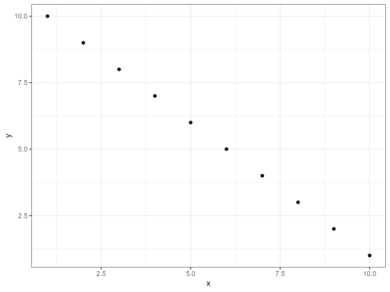
Again, there are a large number of chunk options specific to producing plots and figures. See [here][rmd-ref] for more details.
9.3.4.5 Adding tables
R markdown can print the contents of a dataframe as a table (or any other tabular object such as a summary of model output) by including the name of the dataframe in a code chunk. For example, to create a table of the first 10 rows of the inbuilt dataset iris
```{r, ugly-table}
iris[1:10,]
```
## Sepal.Length Sepal.Width Petal.Length Petal.Width
## 1 5.1 3.5 1.4 0.2
## 2 4.9 3.0 1.4 0.2
## 3 4.7 3.2 1.3 0.2
## 4 4.6 3.1 1.5 0.2
## 5 5.0 3.6 1.4 0.2
## 6 5.4 3.9 1.7 0.4
## 7 4.6 3.4 1.4 0.3
## 8 5.0 3.4 1.5 0.2
## 9 4.4 2.9 1.4 0.2
## 10 4.9 3.1 1.5 0.1
## Species
## 1 setosa
## 2 setosa
## 3 setosa
## 4 setosa
## 5 setosa
## 6 setosa
## 7 setosa
## 8 setosa
## 9 setosa
## 10 setosaBut how ugly is that! You can create slightly nicer looking tables using native markdown syntax (this doesn’t need to be in a code chunk).
    |     x      |    y       |
    |:----------:|:----------:|
    |  1         |   5        |
    |  2         |   4        |
    |  3         |   3        |
    |  4         |   2        |
    |  5         |   1        |
| x | y |
|---|---|
| 1 | 5 |
| 2 | 4 |
| 3 | 3 |
| 4 | 2 |
| 5 | 1 |
The :-------: lets R markdown know that the line above should be treated as a header and the lines below as the body of the table. Alignment within the table is set by the position of the :. To center align use :------:, to left align :------ and right align ------:. Whilst it can be fun(!) to create tables with raw markup it’s only practical for very small and simple tables.
The easiest way we know to include tables in an R markdown document is by using the kable() function from the knitr package (this should have already been installed when you installed the rmarkdown package). The kable() function can create tables for HTML, PDF and Word outputs.
To create a table of the first 10 rows of the iris dataframe using the kable() function simply write your code block as
```{r, kable-table}
library(knitr)
kable(iris[1:10,])
```| Sepal.Length | Sepal.Width | Petal.Length | Petal.Width | Species |
|---|---|---|---|---|
| 5.1 | 3.5 | 1.4 | 0.2 | setosa |
| 4.9 | 3.0 | 1.4 | 0.2 | setosa |
| 4.7 | 3.2 | 1.3 | 0.2 | setosa |
| 4.6 | 3.1 | 1.5 | 0.2 | setosa |
| 5.0 | 3.6 | 1.4 | 0.2 | setosa |
| 5.4 | 3.9 | 1.7 | 0.4 | setosa |
| 4.6 | 3.4 | 1.4 | 0.3 | setosa |
| 5.0 | 3.4 | 1.5 | 0.2 | setosa |
| 4.4 | 2.9 | 1.4 | 0.2 | setosa |
| 4.9 | 3.1 | 1.5 | 0.1 | setosa |
The kable() function offers plenty of options to change the formatting of the table. For example, if we want to round numeric values to one decimal place use the digits = argument. To center justify the table contents use align = 'c' and to provide custom column headings use the col.names = argument. See ?knitr::kable for more information.
```{r, kable-table2}
kable(iris[1:10,], digits = 0, align = 'c',
       col.names = c('sepal length', 'sepal width',
       'petal length', 'petal width', 'species'))
```| sepal length | sepal width | petal length | petal width | species |
|---|---|---|---|---|
| 5 | 4 | 1 | 0 | setosa |
| 5 | 3 | 1 | 0 | setosa |
| 5 | 3 | 1 | 0 | setosa |
| 5 | 3 | 2 | 0 | setosa |
| 5 | 4 | 1 | 0 | setosa |
| 5 | 4 | 2 | 0 | setosa |
| 5 | 3 | 1 | 0 | setosa |
| 5 | 3 | 2 | 0 | setosa |
| 4 | 3 | 1 | 0 | setosa |
| 5 | 3 | 2 | 0 | setosa |
You can further enhance the look of your kable tables using the kableExtra package (don’t forget to install the package first!). See [here][kableExtra] for more details and a helpful tutorial.
```{r, kableExtra-table}
library(kableExtra)
kable(iris[1:10,]) %>%
    kable_styling(bootstrap_options = "striped", font_size = 10)
```| Sepal.Length | Sepal.Width | Petal.Length | Petal.Width | Species |
|---|---|---|---|---|
| 5.1 | 3.5 | 1.4 | 0.2 | setosa |
| 4.9 | 3.0 | 1.4 | 0.2 | setosa |
| 4.7 | 3.2 | 1.3 | 0.2 | setosa |
| 4.6 | 3.1 | 1.5 | 0.2 | setosa |
| 5.0 | 3.6 | 1.4 | 0.2 | setosa |
| 5.4 | 3.9 | 1.7 | 0.4 | setosa |
| 4.6 | 3.4 | 1.4 | 0.3 | setosa |
| 5.0 | 3.4 | 1.5 | 0.2 | setosa |
| 4.4 | 2.9 | 1.4 | 0.2 | setosa |
| 4.9 | 3.1 | 1.5 | 0.1 | setosa |
If you want even more control and customisation options for your tables take a look at the [pander][pander] and [xtable][xtable] packages.
9.3.4.6 Inline R code
Up till now we’ve been writing and executing our R code in code chunks. Another great reason to use R markdown is that we can also include our R code directly within our text. This is known as ‘inline code’. To include your code in your R markdown text you simply write `r write your code here`. This can come in really useful when you want to include summary statistics within your text. For example, we could describe the iris dataset as follows:
Morphological characteristics (variable names:  `r names(iris)[1:4]`) were measured from
`r nrow(iris)` *Iris sp.* plants from  `r length(levels(iris$Species))` different
species. The mean Sepal length was `r round(mean(iris$Sepal.Length), digits = 2)` mm.
which will be rendered as
Morphological characteristics (variable names: Sepal.Length, Sepal.Width, Petal.Length, Petal.Width) were measured from 150 iris plants from 3 different species. The mean Sepal length was 5.84 mm.
The great thing about including inline R code in your text is that these values will automatically be updated if your data changes.
9.3.4.7 Some tips and tricks
Problem :
When rendering my R markdown document to pdf my code runs off the edge of the page.
Solution:
Add a global_options argument at the start of your .Rmd file in a code chunk:
```{r, global_options, include=FALSE}
knitr::opts_chunk$set(message=FALSE, tidy.opts=list(width.cutoff=60), tidy=TRUE)
```
This code chunk won’t be displayed in the final document due to the include = FALSE argument and you should place the code chunk immediately after the YAML header to affect everything below that.
tidy.opts = list(width.cutoff = 60), tidy=TRUE defines the margin cutoff point and wraps text to the next line. Play around with this value to get it right (60-80 should be OK for most documents).
Problem:
When I load a package in my R markdown document my rendered output contains all of the startup messages and/or warnings.
Solution:
You can load all of your packages at the start of your R markdown document in a code chunk along with setting your global options.
```{r, global_options, include=FALSE}
knitr::opts_chunk$set(message=FALSE, warning=FALSE, tidy.opts=list(width.cutoff=60))
suppressPackageStartupMessages(library(ggplot2))
```
The message=FALSE and warning=FALSE arguments suppress messages and warnings. The suppressPackageStartupMessages(library(ggplot2)) will load the ggplot2 package but suppress startup messages.
Problem:
When rendering my R markdown document to pdf my tables and/or figures are split over two pages.
Solution:
Add a page break using the LateX \pagebreak notation before your offending table or figure
Problem:
The code in my rendered document looks ugly!
Solution:
Add the argument tidy=TRUE to your global arguments. Sometimes, however, this can cause problems especially with correct code indentation.
```{r, global_options, include=FALSE}
knitr::opts_chunk$set(message=FALSE, tidy.opts=list(width.cutoff=60), tidy=TRUE)
```
9.3.4.8 Further Information
Although we’ve covered more than enough to get you quite far using R markdown, as with most things R related, we’ve really only had time to scratch the surface. Happily, there’s a wealth of information available to you should you need to expand your knowledge and experience. A good place to start is the excellent free book written by the creator of R markdown Yihui Xie .
Comments
As you can see above the meaning of the
#symbol is different when formatting text in an R markdown document compared to a standard R script (which is used to included a comment - remember?!). You can, however, use a#symbol to comment code inside a code chunk as usual (more about this in a bit). If you want to include a comment in your R markdown document outside a code chunk which won’t be included in the final rendered document then enclose your comment between<!--and-->.